QSP in R
By admin 02-Mar-2024
Author: Anuraag Saini
What do we do?
At Vantage Research, we assist decision-making throughout the drug discovery and development process. We do it via answering questions related to exposure, efficacy, toxicity in preclinical, translational and clinical settings using mechanistic models often represented by ordinary differential equations [1]. These models are quantitatively backed by extensive literature surveys on physiology of a disease, mechanism of action of a drug and are carefully calibrated to clinically relevant readouts.
Why do we do it?
Model informed drug discovery process aims to integrate information from diverse data sources to help decrease both uncertainty and failure rates, and to develop information that cannot or would not be generated experimentally. Mechanistic models, especially QSP, go a level deeper in providing explanations about why or why not some drugs or drug combinations will work better than others.
How do we do it?
Quantitative systems pharmacology (QSP) modeling is a process where physiology of a disease and mechanism of action of a drug are like individual puzzle pieces. QSP solves this puzzle by mathematically connecting molecular to cellular mechanisms, cellular mechanisms to organs, organs to patients level and from patients to populations levels.
We will understand the QSP workflow using a published insulin-regulation model. Although there are a plethora of insulin-glucose regulation models, we chose one published by Contreas et al since it captures important aspects of insulin-glucose regulation and it is structurally simple to implement[2,3].
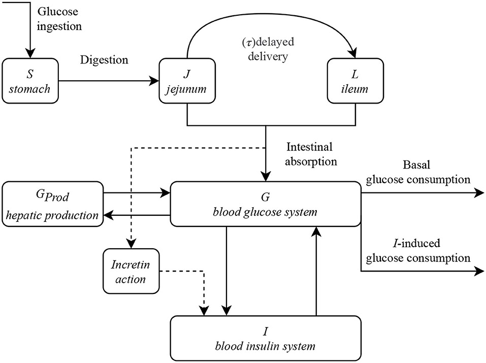
To make things simple, let’s assume I am drinking pineapple juice. Glucose ingestion takes place in the stomach, it travels through the small intestine getting absorbed along the way from Jejunum (middle part of small intestine) to Ileum (end of small intestine).
Absorbed glucose increases my blood glucose levels. I can use this glucose to provide energy to my brain, to carry out basal metabolic functions and to store some of it as glucose reserves for later use.
Insulin plays an important role in regulating blood glucose in the body. The pancreas senses the rising glucose levels in the body and starts producing insulin which then helps glucose to be taken up by muscle for utilization and by liver for storage as glucose reserve, thereby regulating the blood glucose. Insulin’s lack of effectiveness (could be due to insulin secretion deficiency or due to insulin resistance or some combination of both) leads to elevated blood glucose levels which people most commonly known as Diabetes.
Let’s do it together using R!
Required libraries: mrgsolve, ggplot2, lhs, parallel, future, mrgsim.parallel, dplyr
Other required dependencies: Rtools, rstudioapi, rstan
Now that we understand the basics. Let’s do the fun stuff!
We will represent Insulin-Glucose regulation mathematically and use the MRGsolve package [4] in R for simulating a system of equations.
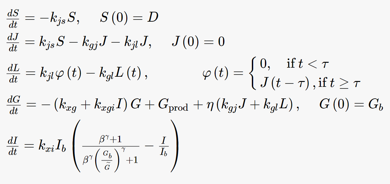
Consider the system of equations in Figure 2 which represents the insulin-glucose regulation (taken from Contreras et al [2]). Let us see how we can represent this system in R and simulate different scenarios using R. In the following exercises, we will see how to (a) Set up the equations in R, (b) Work with delayed ODEs, (c) Add meals as an input to the model, (d) Visualize plasma glucose using 3 meals for 2 days, (e) Input rate constants from excel into R, (f) Perform sensitivity analysis, (g) Top down data that the model will reproduce, (h) Perform a global optimization to reproduce the top down data with minimal error and finally (i) Generate a virtual population
Exercise 1: Make the model
Let us construct a “Glucose-Insulin Regulation Model” using the MRGsolve framework in C++. This model is based on a published model from Contreras et at 2020 [2].
As a best practice, it is ideal to keep the model file separate from the execution code. Following model is saved under filename “GlucoseInsulinRegulation.cpp”. Details about the structure of the model file are discussed in detail in subsequent exercises.
Code
Rcpp
// To use c++ standard function library
[PARAM]
// The parameter list is declared using PARAM block
tou = 80//
kLambda = 0.04// Production rate of glucose from liver
incretin = 3.46// incretin action on glucose
eta = 0.02//bioavailability of absorbed glucose
kSI1 = 0.19// absorption in jejunum from stomach
kI1I2 = 0.043// absorption in Ileum from jejunum
kI1G = 0.13// absorption in PlasmaGlucose from jejunum
kI2G = 0.21// absorption in PlasmaGlucose from Ileum
kGB = 0.016// basal glucose utilization rate from PlasmaGlucose
kGI = 1.37e-7// Insulin dependent glucose utilization rate from PlasmaGlucose
kI = 0.017// insulin degradation rate
beta = 109// Scale for insulin production saturation
gamma = 1.4//Scale for insulin production acceleration
food_amt = 0 // Food intake
Gprod_0 = 4.0; // Basleine prdocution of glucose
PlasmaGlucose_0 = 4.0;
Pls_Ins_0 = 25.8;
[INIT]
// INIT - name and initial value of all the compartments
// Initial conditions
// compartment 1
Stomach = 0 //392.7
// compartment 2
Jejunum= 0.0
// compartment 3
Ileum = 0.0
// compartment 4
PlasmaGlucose = 4.0
// compartment 5
Pls_Ins = 25.8
// compartment 6
Gluc_24hr = 90
[GLOBAL]
// GLOBAL block is used to define Global variables, vectors, etc. that can be used anywhere in other blocks
std::list delayed_Glucose(8);
[MAIN]
// Main block is used to define repeating algebraic calculations.
double PlasmaGlucose_mgdl = PlasmaGlucose*18;
double currMinutes24hr = (TIME-std::floor(TIME/1440)*1440);
double currMinutes10min = (TIME-std::floor(TIME/10)*10);
[TABLE]
// TABLE is used to define repeating algebraic calculations.
if(currMinutes10min==0){ delayed_Glucose.push_back(Jejunum); }
[ODE]
// ODE block is used to define system of ODEs (state nodes) and other repeating algebraic calculations
double Delayed_Ileum = delayed_Glucose.back();
double Gprod = kLambda / (kLambda/Gprod_0 + PlasmaGlucose - PlasmaGlucose_0);
double G_hat = PlasmaGlucose + incretin*(kI1G * Jejunum + kI2G * Ileum);
double Gluc_24hr_Avg_Calculation = (1/1440.0)*(PlasmaGlucose_mgdl-Gluc_24hr);
//// ODEs:
// compartment 1
// Stomach
dxdt_Stomach = - kSI1 * Stomach;
// compartment 2
dxdt_Jejunum = kSI1*Stomach - kI1I2*Jejunum - kI1G*Jejunum;
// compartment 3
dxdt_Ileum = kI1I2*Delayed_Ileum - kI2G*Ileum;
// compartment 4
dxdt_PlasmaGlucose = Gprod + eta * (kI1G * Jejunum + kI2G * Ileum) - kGB*PlasmaGlucose - kGI*Pls_Ins*PlasmaGlucose;
// compartment 5
// Plasma compartment of insulin
dxdt_Pls_Ins = kI*Pls_Ins_0 *((pow(beta,gamma) + 1.0)/((pow(beta,gamma))*pow((PlasmaGlucose/G_hat),gamma) + 1.0) - Pls_Ins/Pls_Ins_0);
// compartment 6
// Proxy for 24-hour average plasma glucose
dxdt_Gluc_24hr = (1/1440.0)*(PlasmaGlucose_mgdl-Gluc_24hr);
[CAPTURE]
// CAPTURE block is used to record the values of the species/nodes other than ODE (state nodes)
Delayed_Ileum Gprod G_hat PlasmaGlucose_mgdl currMinutes10min currMinutes24hr Gluc_24hr_Avg_Calculation
Exercise 2: How to work with delayed ODEs in mrgSolve
Here we want Ileum to follow Jejunum but with a delay of 80 mins. There isn't a standard way of doing this using standard solvers for ordinary differential equations. Hence, we are using a coding trick to solve this issue.
We have created an array of fixed size of 8 elements that will keep storing values every 10 min such that the difference in time between first element and last element is 80 mins. This is initialized under the [GLOBAL] block.
We then create a counter that resets every 10 mins under the [MAIN] block.
Every 10 mins, values of Jejunum are stored in the defined array under the [TABLE] block.
First value of the array is then used for further calculations under the [ODE] block.
Code
[GLOBAL]
std::list delayed_Glucose(8);
[MAIN]
double currMinutes10min = (TIME-std::floor(TIME/10)*10);
[TABLE]
if(currMinutes10min==0){
delayed_Glucose.push_back(Jejunum);
}
[ODE]
double Delayed_Ileum = delayed_Glucose.back();
// compartment 3
dxdt_Ileum = kI1I2*Delayed_Ileum - kI2G*Ileum;
Exercise 3: Set up the model with 3 meals a day
We need to set up an event to add calorie intake in the Stomach. Let's create 3 recurring events for breakfast, lunch and dinner.
These events will require the following
Amount of food : amt
Rate of input (eating) : rate
Time of food intake : time
Repeat interval - this is constant (1440 mins); every 24 hrs : ii
Number of times food intake will be invoked : addl
Code
Code
n_days = 2 #(days)
bf_amt = 450
bf_time = 60
bf_time_interval = 15
lunch_amt = 600
lunch_time = 300
lunch_time_interval = 20
dinner_amt = 800
dinner_time = 660
dinner_time_interval= 30
additional_dose_food = n_days-1
breakfast <- ev(cmt ="Stomach", amt = bf_amt, rate = bf_amt/bf_time_interval, time = bf_time, ii=1440, addl = additional_dose_food)
lunch <- ev(cmt ="Stomach", amt = lunch_amt, rate = lunch_amt/lunch_time_interval, time = lunch_time, ii=1440, addl = additional_dose_food)
dinner <- ev(cmt ="Stomach", amt = dinner_amt, rate = dinner_amt/dinner_time_interval, time = dinner_time, ii=1440, addl = additional_dose_food)
# combine all the events together
Meals <- c(breakfast,lunch,dinner)
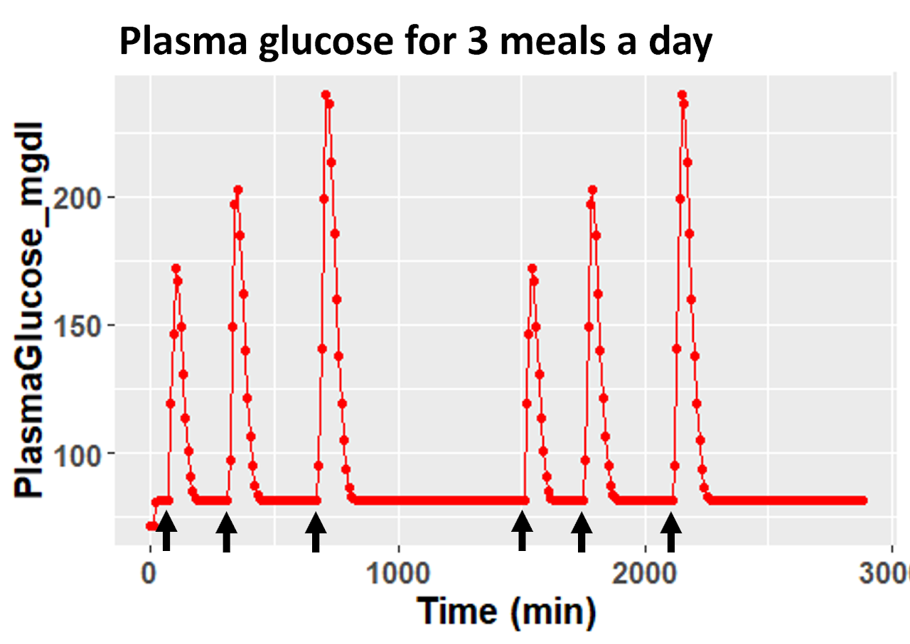
Exercise 4: Visualise plasma glucose for 3 meals for 2 days
We need to compile the c++ model, add food intake information and run the simulation using mrgsim. For more information on the syntax visit mrgsolve user guide and ggplot documentation.
Code
file.model <- "GlucoseInsulinRegulation.cpp"
mod <- mread(file.model)
model_output <- mrgsim(mod,Meals,end=(n_days*1440),delta=10)
# Plot PlasmaGlucose_mgdl
sims = as.data.frame(model_output)
node_sims = "PlasmaGlucose_mgdl"
ylabel = "PlasmaGlucose_mgdl"
ggplot() +
geom_line(aes(y=sims[,node_sims],x=(sims[,"time"])/60), colour="red") + # first layer
geom_point(aes(y=sims[,node_sims],x=(sims[,"time"])/60), colour="red") +
theme(text = element_text(size=15,face='bold')) +
xlab('Time (hours)') +
ylab(ylabel) +
ggtitle(paste("Plasma glucose for 3 meals a day"))
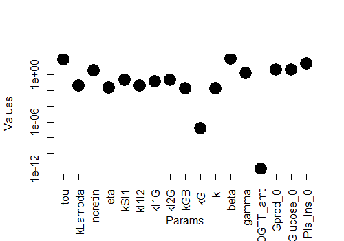
Exercise 5: Reading and visualising the data/excel files
Now, we have the model set up. Let's read an excel file with values of parameters (or input rate constants) defined in [PARAM] block and plot the values of each parameter. Parameter values and units are directly taken from Contreras et at 2020 [2].
Code
file.params = "ModelParams.csv"
# Load params as data frame
param_df = as.data.frame(read.csv(file.params))
# Converting data frame to list
param_data = setNames(data.frame(t(param_df[,2])),param_df[,1])
# Plot the params
plot(t(param_data),xlab= "Params", ylab = "Values", pch =19, cex = 2.5,log="y",xaxt = "n")
# pch : for marker shape
# cex : for marker size
# log = “y” : for converting y axis to log
# xaxt = “n”: remove the x-labels
# Add custom x-labels
xticks <- colnames(param_data)
axis(side=1, at=1:17, labels = xticks, las = 2)
# las = 2: for rotating labels by 90 degrees
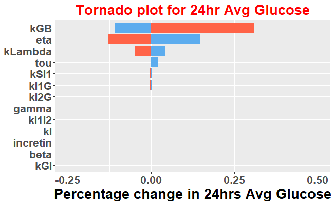
Exercise 6: Perform a sensitivity analysis of parameters and visualise using tornado plot
Sensitivity analysis can differentiate the model parameters that change the output significantly vs those which have minimal impact on the model output. Here we will evaluate the sensitivity of the parameters on 24hr avg glucose by changing the parameter values 50% up and down from their baseline values. It is important to run the model to steady state before performing this evaluation. Hence we will run the model to 150 days before performing sensitivity analysis.
Code
## Run the model for 150 days
# Specify the meals for 150 days
n_days <- 150
additional_dose_food = n_days-1
breakfast <- ev(cmt ="Stomach", amt = bf_amt, rate = bf_amt/bf_time_interval, time = bf_time, ii=1440, addl = additional_dose_food)
lunch <- ev(cmt ="Stomach", amt = lunch_amt, rate = lunch_amt/lunch_time_interval, time = lunch_time, ii=1440, addl = additional_dose_food)
dinner <- ev(cmt ="Stomach", amt = dinner_amt, rate = dinner_amt/dinner_time_interval, time = dinner_time, ii=1440, addl = additional_dose_food)
# combine all the events together
Meals <- c(breakfast,lunch,dinner)
## Get parameters to perform sensitivity on
num_params = length(param_data)-4
param_names_to_vary <- colnames(param_data)[1:num_params]
model_output <- mrgsim(mod,Meals,end=(n_days*1440),delta=10)
## Get mean value of Plasma Glucose from 24 hrs data points for baseline
rTotal = length(model_output$Gluc_24hr)
avgVal = mean(model_output$Gluc_24hr[rTotal-1440:rTotal])
## Specify how much the parameters should vary
foldChange = 0.5
perChange = matrix(nrow=num_params,ncol=2)
LB_avgVal = matrix(nrow=num_params,ncol=6)
UB_avgVal = matrix(nrow=num_params,ncol=6)
## Run the model for each parameters
ii=1
for(ii in 1:num_params){
print(cbind(param_data[ii]*(1-foldChange), param_data[ii]*(1+foldChange)))
## For lower value
mod % param(param_data[ii]*(1-foldChange))
output_LB <- mrgsim(mod,Meals,end=(n_days*1440),delta=10)
LB_avgVal[ii,] = mean(output_LB$Gluc_24hr[rTotal-1440:rTotal])
## For higher value
mod % param(param_data[ii]*(1+foldChange))
output_UB <- mrgsim(mod,end=(n_days*1440),Meals,delta=10)
UB_avgVal[ii,] = mean(output_UB$Gluc_24hr[rTotal-1440:rTotal])
lb <- (LB_avgVal[ii,] - avgVal)/avgVal
ub <- (UB_avgVal[ii,] - avgVal)/avgVal
perChange[ii,] = c(lb[which.max(abs(lb))], ub[which.max(abs(ub))])
## Plot both lower and higher output
par(mfrow=c(2,1))
plot(output_LB$time, output_LB$Gluc_24hr)
plot(output_UB$time, output_UB$Gluc_24hr)
mtext(param_names_to_vary[ii],side = 3,line = - 2,outer = TRUE)
mod % param(param_data)
}
## Setting up the dataframe for plots
per_change_LB2 <- data.frame(param_names_to_vary,rep(1,num_params),perChange[,1])
per_change_LB2 <- per_change_LB2[order(abs(per_change_LB2[,3]),decreasing=TRUE),]
colnames(per_change_LB2)[3] <- "per_change"
colnames(per_change_LB2)[2] <- "ID"
per_change_UB2 <- data.frame(param_names_to_vary,rep(2,num_params),perChange[,2])
per_change_UB2 <- per_change_UB2[order(abs(per_change_UB2[,3]),decreasing=TRUE),]
colnames(per_change_UB2)[3] <- "per_change"
colnames(per_change_UB2)[2] <- "ID"
## Plot tornado plot for sensitivity analysis
data <- data.frame(rbind(per_change_LB2,per_change_UB2))
ggplot(data)+ #,aes(x=hr,y=Pls_GCG_Conc,col=ID))+
geom_bar(aes(x=reorder(param_names_to_vary,abs(-per_change)),y=per_change),stat='identity',position='identity', col=as.factor(data$ID),fill=c(rep("tomato",num_params),rep("steelblue2",num_params)),lty="blank")+
ylab(paste0("Percentage change in 24hrs Avg Glucose"))+
xlab(NULL) +
ylim(c(-0.25,0.5))+
ggtitle(paste0("Tornado plot for 24hr Avg Glucose"))+
theme(plot.title = element_text(color = "red", size = 20, hjust = 0.5),legend.title = element_blank())+
theme(text = element_text(size=20)) +
theme(text=element_text(face="bold"))+
theme(legend.position="bottom")+
coord_flip()
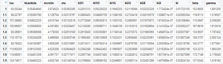
Exercise 7: Create and visualise a virtual cohort
Creating a virtual cohort means creating multiple patients that have different parameterizations such that their steady state values differ from each other. This is useful if you want to re-create a clinical trial and try to match baseline characteristics with mean and std dv from observed data. In this example, we will try to create 10 VPs with different 24hr Avg Glucose values. To achieve this, we will vary the parameters randomly between their lower and upper bounds to create 10 parameterizations or virtual patients for the model to run.
Visualize the parameter combinations to generate a virtual cohort
Code
cohort_size = 10
num_params = length(param_data)-4
param_names_to_vary <- colnames(param_data)[1:num_params]
param_cohort <- param_data[rep(seq_len(nrow(param_data)),cohort_size),]
chosen_inds<-match(param_names_to_vary,param_table$Name)
LB_params = rep(0.3,num_params)
UB_params = rep(0.3,num_params)
rand_sample <- randomLHS(cohort_size,num_params)
# parameters set for all VPs - each row representing one VP
param_cohort[,chosen_inds] <- t((param_table[chosen_inds,2]) +
((param_table[chosen_inds,2])*(1+UB_params) - (param_table[chosen_inds,2])*(1-LB_params))*t(rand_sample))
#View parameter combinations that represent a cohort
View(param_cohort)
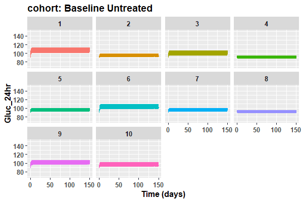
Formatting the parameter combinations to run them in parallel and plot 24hr average glucose for 10 VPs at steady state. For more information on syntax for parallelization refer to the documentation.
Code
param_cohort <- cbind(param_cohort,ID=1:nrow(param_cohort))
# Slice the dataset (parameter combinations) to run them in parallel
idata <- split(param_cohort, param_cohort$ID)
future::plan(future::multisession, workers = 2L)
out <- fu_mrgsim_ei(mod, Meals, idata,end=(n_days*1440),delta=10,.seed = 123, nchunk = 6)
# Annotate simulation output for plotting
results = as.data.frame(out)
# remove invalid VPs from results, if any
invalid_ID <- (unique(results$ID[is.nan(results$Gluc_24hr)]))
results = results[!(results$ID %in% invalid_ID),]
# keep unique time points for each ID
results % distinct(time, ID, .keep_all=TRUE)
plots <- function(y_axis_value,y_axis_name,sims,ylow,yhigh){
(ggplot(data = sims)+
geom_line(aes(x=(sims[,"time"]/1440),y=sims[,y_axis_value],color=as.factor(sims[,"ID"])))+
facet_wrap(~ sims[,"ID"]) +
theme(text = element_text(size=12,face='bold'),legend.position = "none") +
xlab('Time (days)') +
ylab(y_axis_name) +
ylim(ylow,yhigh)+
ggtitle(paste("cohort: Baseline Untreated")) )}
print(dose_plot_cohort <- plots(sims=results,y_axis_value="Gluc_24hr",y_axis_name="Gluc_24hr",ylow=70,yhigh=150))
Acknowledgments
Thank you Shaifali Saroha and Tanvi Joshi for collaborating on the code.
Access the following files here (a) Model file: GlucoseInsulinRegulation.cpp, (b) Simulation file: RunModel.R and (c) Parameter file: ModelParams.csv.
https://drive.google.com/drive/folders/1SWLgCO6DuKT6-dzAc22RsX1j3s6jAdSf
References
1. Allerheiligen, S.R.B. (2010), Next-Generation Model-Based Drug Discovery and Development: Quantitative and Systems Pharmacology. Clinical Pharmacology & Therapeutics, 88: 135-137. https://doi.org/10.1038/clpt.2010.81
2. Contreras, Sebastián, et al. “A novel synthetic model of the glucose-insulin system for patient-wise inference of physiological parameters from small-size OGTT data.” Frontiers in bioengineering and biotechnology 8 (2020): 195. https://doi.org/10.3389/fbioe.2020.00195
3.Ajmera, I., Swat, M., Laibe, C., Le Novère, N., & Chelliah, V. (2013). The impact of mathematical modeling on the understanding of diabetes and related complications. CPT: pharmacometrics & systems pharmacology, 2(7), e54. https://doi.org/10.1038/psp.2013.30.
4. Baron K (2023). mrgsolve: Simulate from ODE-Based Models. R package version 1.0.9. https://github.com/metrumresearchgroup/mrgsolve.
About the Author